Leaky Joins
Ying Yang, Oliver Kennedy
Leaky Joins
Ying Yang, Oliver Kennedy

Disclaimer
Ying could not be here today. If you like her ideas, get in touch with her.
(If you don't, blame my presentation)
(Also, Ying is on the job market)
(not immediately relevant to the talk, but you should check it out)
Roughly 1-2 years ago...
Ying: To implement {cool feature in Mimir}, we'll need to be able to perform inference on Graphical Models, but we will not know how complex they are.
Graphical Models
Joint probability distributions are expensive to store
$$p(D, I, G, S, J)$$
Bayes rule lets us break apart the distribution
$$= p(D, I, G, S) \cdot p(J | D, I, G, S)$$
And conditional independence lets us further simplify
$$= p(D, I, G, S) \cdot p(J | G, S)$$
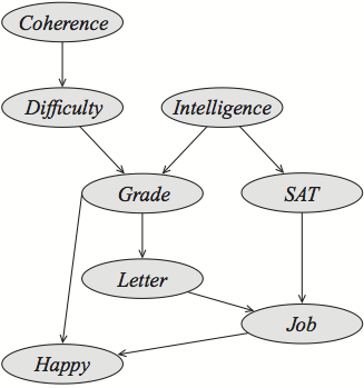
This is basis for a type of graphical model called a "Bayes Net"
Bayesean Networks
$p(D=1, I=0, S=0, G=2, J=1)$
$=\;0.5$
$\cdot\;0.7$
$\cdot\;0.95$
$\cdot\;0.25$
$\cdot\;0.8$
$=\;0.0665$
$p(D,I,S,G,J)$
$=$
$p(D) \bowtie p(I) \bowtie p(S|I) \bowtie p(G|D,I) \bowtie p(J|G,S)$
Inference
$p(J) = \sum_{D,I,S,G}p(D,I,S,G,J)$
(aka the computing the marginal probability)Inference Algorithms
- Exact (e.g. Variable Elimination)
- Fast and precise, but scales poorly with graph complexity.
- Approximate (e.g. Gibbs Sampling)
- Consistent performance, but only asymptotic convergence.
Key Challenge: For {really cool feature} we don't know whether we should use exact or approximate inference.
Can we gracefully degrade from exact to approximate inference?
	SELECT J.J, SUM(D.p * I.p * S.p * G.p * J.p) AS p
	FROM D NATURAL JOIN I NATURAL JOIN S
	       NATURAL JOIN G NATURAL JOIN J
	GROUP BY J.J
(Inference is essentially a big group-by aggregate join query)
(Variable elimination is Aggregate Pushdown + Join Ordering)
Idea: Online Aggregation
Online Aggregation (OLA)
$Avg(3,6,10,9,1,3,9,7,9,4,7,9,2,1,2,4,10,8,9,7) = 6$
$Avg(3,6,10,9,1) = 5.8$ $\approx 6$
$Sum\left(\frac{k}{N} Samples\right) \cdot \frac{N}{k} \approx Sum(*)$
Sampling lets you approximate aggregate values with orders of magnitude less data.
Typical OLA Challenges
- Birthday Paradox
- $Sample(R) \bowtie Sample(S)$ is likely to be empty.
- Stratified Sampling
- It doesn't matter how important they are to the aggregate, rare samples are still rare.
- Replacement
- Does the sampling algorithm converge exactly or asymptotically?
Replacement
- Sampling Without Replacement
- ... eventually converges to a precise answer.
- Sampling With Replacement
- ... doesn't need to track what's been sampled.
- ... produces a better behaved estimate distribution.
OLA over GMs
- Tables are Small
- Compute, not IO is the bottleneck.
- Tables are Dense
- Birthday Paradox and Stratified Sampling irrelevant.
- Queries have High Tree-Width
- Intermediate tables are large.
Classical OLA techniques aren't entirely appropriate.
(Naive) OLA: Cyclic Sampling
A Few Quick Insights
- Small Tables make random access to data possible.
- Dense Tables mean we can sample directly from join outputs.
- Cyclic PRNGs like Linear Congruential Generators can be used to generate a randomly ordered, but non-repeating sequence of integers from $0$ to any $N$ in constant memory.
Linear Congruential Generators
If you pick $a$, $b$, and $N$ correctly, then the sequence:
$K_i = (a\cdot K_{i−1}+b)\;mod\;N$
will produce $N$ distinct, pseudorandom integers $K_i \in [0, N)$
Cyclic Sampling
To marginalize $p(\{X_i\})$...
- Init an LCG with a cycle of $N = \prod_i |dom(X_i)|$
- Use the LCG to sample $\{x_i\} \in \{X_i\}$
- Incorporate $p(x_i = X_i)$ into the OLA estimate
- Repeat from 2 until done
Accuracy
- Sampling with Replacement
- Chernoff Bounds, Hoeffding Bounds give an $\epsilon-\delta$ guarantee on the sum/avg of a sample with replacement.
- Without Replacement?
- Serfling et. al. have a variant of Hoeffding Bounds for sampling without replacement.
Cyclic Sampling
- Advantages
- Progressively better estimates over time.
- Converges in bounded time.
- Disadvantages
- Exponential time in the number of variables.
Better OLA: Leaky Joins
Make Cyclic Sampling into a composable operator

| $G$ | # | $\sum p_{\psi_2}$ |
|---|---|---|
| 1 | 1 | 0.126 |
| $I$ | $G$ | # | $\sum p_{\psi_1}$ |
|---|---|---|---|
| 0 | 1 | 1 | 0.18 |
| $G$ | # | $\sum p_{\psi_2}$ |
|---|---|---|
| 1 | 3 | 0.348 |
| 2 | 4 | 0.288 |
| 3 | 4 | 0.350 |
| $I$ | $G$ | # | $\sum p_{\psi_1}$ |
|---|---|---|---|
| 0 | 1 | 2 | 0.140 |
| 1 | 1 | 2 | 0.222 |
| 0 | 2 | 2 | 0.238 |
| 1 | 2 | 2 | 0.050 |
| 0 | 3 | 2 | 0.322 |
| 1 | 3 | 2 | 0.028 |
| $G$ | # | $\sum p_{\psi_2}$ |
|---|---|---|
| 1 | 4 | 0.362 |
| 2 | 4 | 0.288 |
| 3 | 4 | 0.350 |
| $I$ | $G$ | # | $\sum p_{\psi_1}$ |
|---|---|---|---|
| 0 | 1 | 2 | 0.140 |
| 1 | 1 | 2 | 0.222 |
| 0 | 2 | 2 | 0.238 |
| 1 | 2 | 2 | 0.050 |
| 0 | 3 | 2 | 0.322 |
| 1 | 3 | 2 | 0.028 |
Leaky Joins
- Build a normal join/aggregate graph as in variable elimination: One Cyclic Sampler for each Join+Aggregate.
- Keep advancing Cyclic Samplers in parallel, resetting their output after every cycle so samples "leak" through.
- When the sampler completes one full cycle with a complete input, mark it complete and stop sampling it.
- Continue until a desired accuracy is reached or all tables marked complete.
There's a bit of extra math to compute $\epsilon-\delta$ bounds by adapting Serfling's results. It's in the paper.
Experiments
- Microbenchmarks
- Fix time, vary domain size, measure accuracy
- Fix domain size, vary time, measure accuracy
- Vary domain size, measure time to completion
- Macrobenchmarks
- 4 graphs from the bnlearn Repository
Microbenchmarks
Student: A common benchmark graph.
Accuracy vs Domain
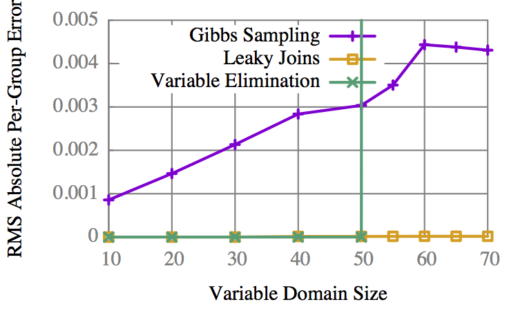
VE is binary: It completes, or it doesn't.
Accuracy vs Time
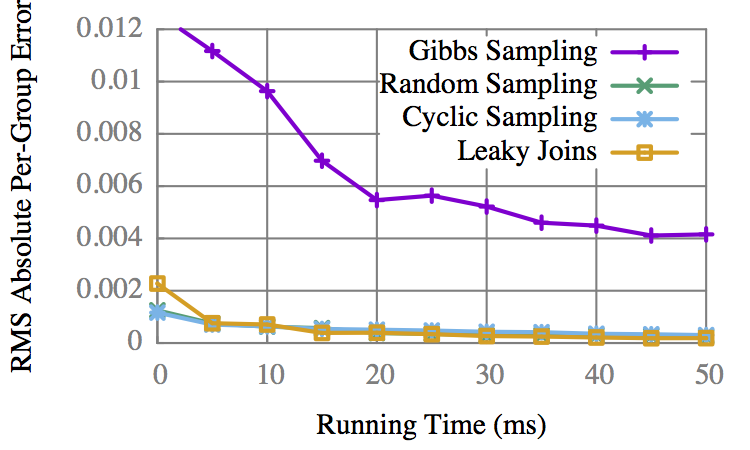
CS gets early results faster, but is overtaken by LJ.
Domain vs Time to 100%
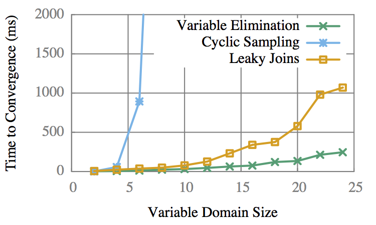
LJ is only 3-5x slower than VE.
"Child"
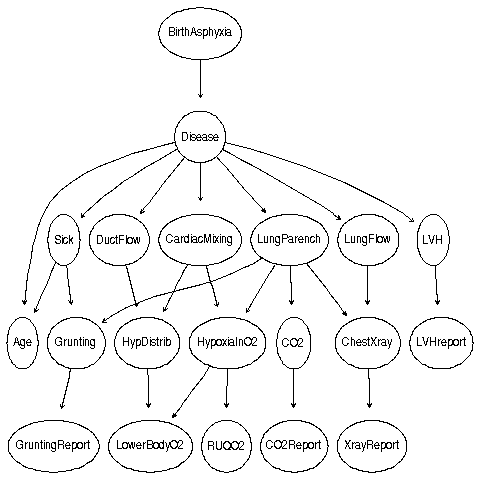
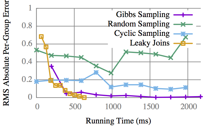
LJ converges to an exact result before Gibbs gets an approx.
"Insurance"
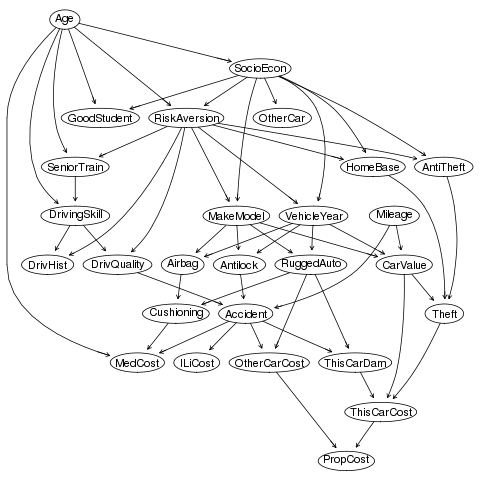
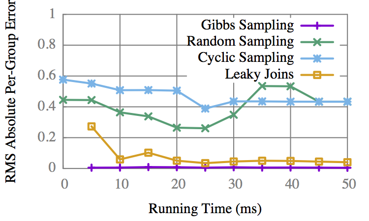
On some graphs Gibbs is better, but only marginally.
More graphs in the paper.
Leaky Joins
- Classical OLA isn't appropriate for GMs.
- Idea 1: LCGs can sample without replacement.
- Idea 2: "Leak" samples through a normal join graph.
- Compared to both Variable Elim. and Gibbs Sampling, Leaky Joins are often better and never drastically worse.
Questions?